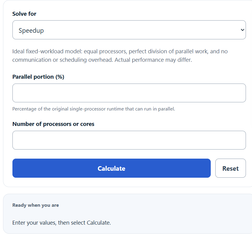
Calculate Amdahl’s Law speedup, maximum speedup, or processors needed from the parallel portion and number of processors or cores.
Related Calculators
- Call Attempts Per Second Calculator
- RTT Calculator
- Log Base 2 Calculator
- Percent To Ratio Calculator
- All Math and Numbers Calculators
Amdahl’s Law Formula
Amdahl’s Law estimates how much faster a task can run when only part of the work can be parallelized. The serial part still runs on one processor, so it limits the total speedup.
- S = speedup compared with running on one processor
- p = parallel portion of the program, entered as a decimal in the formula
- n = number of processors or cores
- 1 – p = serial portion of the program
For maximum theoretical speedup, the processor count approaches infinity. The parallel part becomes negligible, but the serial part remains.
- S_max = maximum possible speedup as processor count becomes very large
- p = parallel portion of the program as a decimal
To find how many processors are needed for a target speedup, the standard Amdahl’s Law equation is rearranged to solve for n.
- n = processors needed
- S = target speedup
- p = parallel portion of the program as a decimal
The speedup function uses the parallel percentage and processor count to estimate ideal speedup. The max speedup function shows the upper limit caused by the serial portion. The processors needed function rounds up to the minimum whole core count for a target speedup under the ideal model. A target of 1 needs only one core; targets at a finite theoretical ceiling cannot be reached with a finite count.
Parallel Portion and Theoretical Speedup Limits
The serial portion has a large effect on the maximum possible gain. Even a small serial fraction can cap speedup sharply.
| Parallel portion | Serial portion | Maximum speedup |
|---|---|---|
| 50% | 50% | 2.00× |
| 75% | 25% | 4.00× |
| 90% | 10% | 10.00× |
| 95% | 5% | 20.00× |
| 99% | 1% | 100.00× |
Speedup Interpretation
| Calculated speedup | Interpretation |
|---|---|
| Less than 1.5× | Less than 1.5 times the single-processor performance; this alone does not identify a bottleneck. |
| 1.5× to 3× | Modest parallel gain. |
| 3× to 8× | Three to eight times the single-processor performance; efficiency also depends on processor count. |
| 8× to 20× | Eight to twenty times the single-processor performance under this ideal model. |
| More than 20× | A very high parallel fraction is required. |
Example Calculations
Example 1: Speedup with 80% parallel code and 8 cores
Suppose a program is 80% parallel and runs on 8 cores.
The expected speedup is 3.33×.
Example 2: Maximum speedup with 95% parallel code
Suppose a program is 95% parallel. The serial portion is 5%.
The maximum theoretical speedup is 20×, no matter how many processors are added.
FAQ
What does the parallel portion mean?
The parallel portion is the fraction of the program that can be split across multiple processors. For example, if 90% of the runtime can be parallelized, then p = 0.90. The remaining 10% is serial and must run sequentially.
Why does adding more processors eventually stop helping much?
Adding processors only speeds up the parallel part. The serial part does not shrink as more processors are added. As the processor count grows, the serial portion becomes the main limit on total speedup.
Can Amdahl’s Law predict real-world performance exactly?
No. Amdahl’s Law is a theoretical estimate. Real systems can be slower because of communication overhead, memory bandwidth limits, synchronization, load imbalance, and scheduling costs. It is best used to understand the upper limit of parallel speedup.