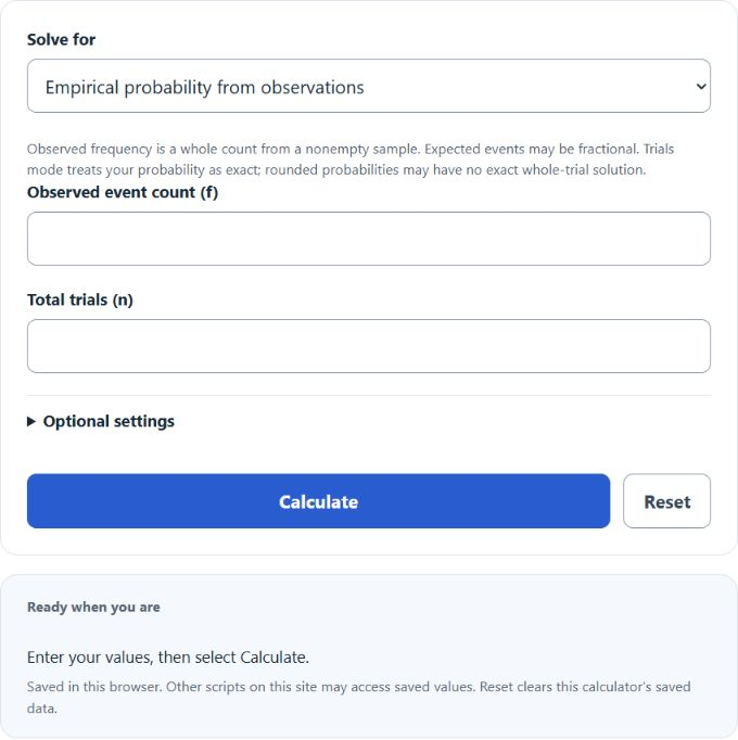
Calculate empirical probability from observed occurrences and total trials, predict expected events, and compare with theoretical probability.
- All Statistics Calculators
- Dice Probability Calculator
- Compound Probability Calculator
- Overlapping Probability Calculator
Empirical Probability Formula
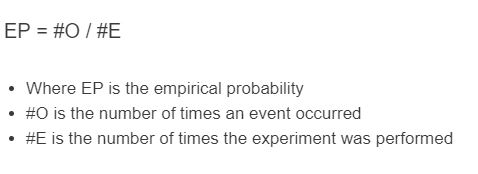
Empirical probability is the ratio of how often an event actually happened to how many times you ran the trial.
- P(E) = empirical probability of event E
- f = frequency (number of times E occurred)
- n = total number of trials
The calculator also supports two related modes:
Use Expected events mode, or the optional future-trials input in probability mode, to calculate the modeled mean in N future trials. The expected count may be fractional and is not a guaranteed outcome.
The optional theoretical-probability input in probability mode compares the observed ratio with a supplied probability; the result is shown in percentage points. Exact trials mode also solves n = f / P when a positive whole-trial solution exists; it does not round a noninteger into an exact observed count.
Observed counts require a positive whole n and whole f with 0 ≤ f ≤ n. The ratio itself is descriptive and does not require independent trials. Population inference and future projections need a suitable sample and stable probabilities; small samples and selection bias can mislead.
Reference Tables
Illustrative normal-approximation margins near probability 0.5 (95% confidence): 1.96 × sqrt(0.5 × 0.5 / n). Percent values here mean percentage points. The normal approximation is poor for small counts or probabilities near 0 or 1; the reliability labels are informal and do not assess sampling bias.
| Trials (n) | Margin of Error | Reliability |
|---|---|---|
| 10 | ±31% | Very weak |
| 30 | ±18% | Weak |
| 100 | ±10% | Moderate |
| 500 | ±4.4% | Good |
| 1,000 | ±3.1% | Strong |
| 10,000 | ±1.0% | Very strong |
How to read a probability value:
| P(E) | Percent | Interpretation |
|---|---|---|
| 0.00 – 0.05 | 0 – 5% | Very rare |
| 0.05 – 0.25 | 5 – 25% | Uncommon |
| 0.25 – 0.50 | 25 – 50% | Less than even |
| 0.50 – 0.75 | 50 – 75% | More likely than not |
| 0.75 – 0.95 | 75 – 95% | Likely |
| 0.95 – 1.00 | 95 – 100% | Almost certain |
Example and FAQ
Example. You flip a coin 80 times and get 34 heads. The empirical probability of heads is 34 / 80 = 0.425, or 42.5%. The theoretical probability is 0.5, so your sample is running about 7.5 percentage points low. With only 80 flips, that gap is well inside normal random variation.
How is empirical probability different from theoretical? Theoretical probability comes from the structure of the situation (a fair die has P = 1/6 for any face). Empirical probability comes from counting what actually happened.
How many trials do I need? Required sample size depends on the precision, confidence level, probability and sampling design. There is no universal minimum of 30. Under the same independent-sampling assumptions, quadrupling n approximately halves the standard error.
Can the result be 0 or 1? Yes. If the event never occurred, P = 0. If it occurred every trial, P = 1. Both are signals to collect more data before drawing conclusions.
Why doesn’t my empirical probability match the theoretical one? Random variation can cause a difference, but so can a biased sample or an incorrect theoretical model. For independent trials with a stable probability, the Law of Large Numbers describes convergence as n grows, not a guarantee for a particular sample.