Calculate Jarque-Bera test statistics, p-values, or solve for skewness, kurtosis, and sample size from the JB formula and decision rule.
Customize This Calculator
Build your own version. Describe what you want changed, added, or compared.
- All Miscellaneous Calculators
- Coefficient of Skewness Calculator
- T Statistic Calculator (T-Value)
- Normality To Percent Calculator
JB Test Formula
The Jarque-Bera (JB) test measures how far a sample departs from normality by combining skewness and kurtosis into a single statistic. It is commonly used for dataset screening and residual analysis when you want a quick numerical check for normal-distribution behavior.
- JB = Jarque-Bera test statistic
- n = sample size
- SK = sample skewness coefficient
- b2 = kurtosis coefficient
The formula compares your sample to the two key benchmarks of a normal distribution:
- Normal skewness = 0
- Normal kurtosis = 3
If both values are close to their normal targets, the JB statistic stays small. If skewness, kurtosis, or both move away from those targets, the JB statistic increases.
What the JB Test Measures
| Input | Meaning | Normal Benchmark |
|---|---|---|
| Sample size (n) | Number of observations used to compute the moments | — |
| Skewness (SK) | Measures asymmetry in the distribution | 0 |
| Kurtosis coefficient (b2) | Measures tail weight and peak shape | 3 |
| JB statistic | Combined normality test statistic | 0 for a perfectly normal sample |
How to Use the Calculator
- Enter the sample size.
- Enter the sample skewness.
- Enter the kurtosis coefficient.
- Read the resulting JB statistic.
- Interpret the result by comparing it to a chi-square reference with 2 degrees of freedom or by converting it to a p-value.
A smaller JB value suggests the sample is closer to normal. A larger value suggests stronger evidence against normality.
Important Input Note
The formula uses the kurtosis coefficient, not excess kurtosis. If your software reports excess kurtosis g2, convert it first:
For example, if excess kurtosis is 0.5, then the kurtosis coefficient entered into the calculator should be 3.5.
Decision Rule
For large samples, the JB statistic is commonly compared to a chi-square distribution with 2 degrees of freedom.
You can also express the significance level through a p-value:
Common reference cutoffs are:
| Significance Level | Critical Value | Interpretation |
|---|---|---|
| 10% | 4.605 | Reject normality if JB is greater than 4.605 |
| 5% | 5.991 | Reject normality if JB is greater than 5.991 |
| 1% | 9.210 | Reject normality if JB is greater than 9.210 |
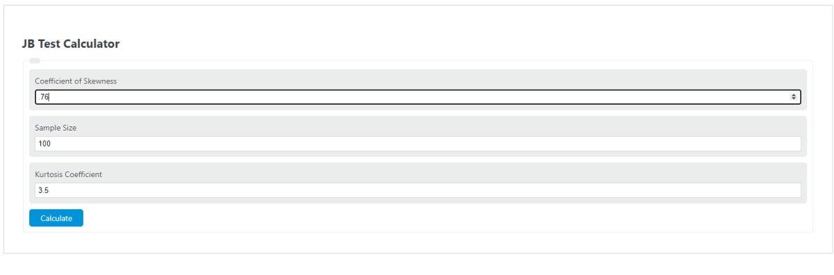
Example
Suppose a sample has:
- Sample size = 100
- Skewness = 0.76
- Kurtosis coefficient = 3.5
Substitute the values into the formula:
Because 10.6683 is greater than 5.991, this sample would typically be considered inconsistent with normality at the 5% level.
How to Interpret the Result
- JB near 0: the sample’s skewness and kurtosis are close to normal-distribution values.
- Moderate JB: some departure from normality may be present.
- Large JB: stronger evidence that the sample is not normally distributed.
- Large sample sizes make the test more sensitive, so even small departures can produce rejection.
When the JB Test Is Most Useful
- Checking whether regression residuals are approximately normal
- Comparing multiple datasets for normality screening
- Identifying whether tail behavior or asymmetry may affect downstream analysis
- Supporting decisions about transformations or nonparametric methods
Common Mistakes
- Entering excess kurtosis instead of the full kurtosis coefficient
- Assuming the test proves a distribution is normal rather than simply failing to reject normality
- Ignoring outliers, which can heavily influence skewness and kurtosis
- Relying only on JB in very small samples instead of also reviewing plots such as histograms or Q-Q plots
This calculator is best used as a fast way to compute the Jarque-Bera statistic from sample size, skewness, and kurtosis so you can quickly judge whether your data appear reasonably normal.