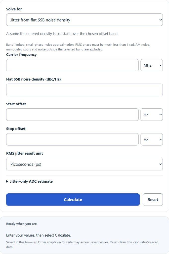
Convert flat-band or integrated phase noise to RMS timing jitter, reverse jitter to integrated noise, and estimate phase error, cycles, and jitter-limited ADC SNR.
Phase Noise to Jitter Formula
Under the small-phase-noise approximation (RMS phase much less than 1 radian), integrate single-sideband (SSB) phase noise over the application’s offset band. Twice that linear one-sideband area gives the approximate RMS phase variance; divide its square root by the carrier’s angular frequency to obtain RMS time jitter:
Flat mode assumes a constant SSB density in dBc/Hz across an integration bandwidth \(\Delta f\). Integrated mode instead accepts the total one-sideband area in dBc, and reverse mode converts band-limited RMS jitter back to that integrated area. The following flat-noise expression gives the optional 6σ span, rather than the calculator’s primary RMS result:
Variables:
- \(L(f)\) is the SSB phase noise in dBc/Hz at offset frequency \(f\) (a power ratio per 1 Hz bandwidth)
- \(f_0\) is the carrier frequency (Hz)
- \(f_1\) to \(f_2\) define the offset-frequency integration limits (Hz), and \(\Delta f = f_2-f_1\) for a flat-noise approximation
- \(J_{pp}\approx 6\sigma_t\) is a common “6σ” peak-to-peak estimate (≈ ±3σ) for Gaussian random jitter; true peak-to-peak of a Gaussian process is unbounded. Observed extremes depend on sample count and observation time; a probability or BER target needs its own model, not a fixed 6σ guarantee
To calculate jitter, convert SSB density from dBc/Hz to a linear power ratio per hertz and integrate over the chosen band. Multiply that one-sideband area by 2 before taking the square root to obtain RMS phase jitter (rad), then divide by 2π times the carrier frequency for RMS time jitter. An integrated input in dBc is already the total one-sideband area, not a density. Flat or integrated inputs do not model AM noise, unmodeled spurs or noise outside the stated band. The optional 6σ value is a qualified Gaussian span, not a measured peak-to-peak bound.
The optional ADC estimate uses SNR = −20log10(2π fin σt), where fin is the analog sinusoidal input frequency, which can differ from the clock carrier. It is a small timing-error, jitter-only estimate; quantization, thermal noise, distortion and other clock or aperture jitter are excluded. Independent jitter sources can be combined by root-sum-square before use; correlated sources require a different model. See Analog Devices’ phase-noise conversion tutorial, aperture-jitter SNR derivation and Keysight’s random-jitter measurement explanation.
| Phase Noise (dBc/Hz) | Jitter for Δf = 1 kHz (ps) | Jitter for Δf = 10 kHz (ps) | Jitter for Δf = 100 kHz (ps) |
|---|---|---|---|
| -60 | 42.7 | 135 | 427 |
| -65 | 24.0 | 75.9 | 240 |
| -70 | 13.5 | 42.7 | 135 |
| -75 | 7.59 | 24.0 | 75.9 |
| -80 | 4.27 | 13.5 | 42.7 |
| -85 | 2.40 | 7.59 | 24.0 |
| -90 | 1.35 | 4.27 | 13.5 |
| -95 | 0.759 | 2.40 | 7.59 |
| -100 | 0.427 | 1.35 | 4.27 |
| -105 | 0.240 | 0.759 | 2.40 |
| -110 | 0.135 | 0.427 | 1.35 |
| -115 | 0.0759 | 0.240 | 0.759 |
| -120 | 0.0427 | 0.135 | 0.427 |
| -125 | 0.0240 | 0.0759 | 0.240 |
| -130 | 0.0135 | 0.0427 | 0.135 |
| -135 | 0.00759 | 0.0240 | 0.0759 |
| -140 | 0.00427 | 0.0135 | 0.0427 |
| -145 | 0.00240 | 0.00759 | 0.0240 |
| -150 | 0.00135 | 0.00427 | 0.0135 |
| -155 | 0.000759 | 0.00240 | 0.00759 |
| Assumptions: flat (single-point) approximation over integration bandwidth Δf; carrier frequency f₀ = 1 GHz; Jitterpp ≈ 6 × σt. Formula: Jitterpp = (6/(2π f₀)) × √(2 × 10^(L/10) × Δf). | |||
What is Phase Noise?
Phase noise is the frequency-domain representation of random fluctuations in the phase of a waveform, and it is related to time-domain jitter. It is a key parameter in the characterization of oscillators and timing components in electronic systems, affecting the performance of communication systems, radars, and other sensitive equipment.
How to Calculate Jitter from Phase Noise?
The following steps outline how to calculate jitter from phase noise:
- Determine the phase noise \(L(f)\) in dBc/Hz as a function of offset frequency.
- Choose an offset-frequency integration range \(f_1\) to \(f_2\) (Hz) that matches your application (or an equivalent integration bandwidth \(\Delta f\) for a simplified approximation).
- Convert the phase noise to linear scale using: \(L_\text{lin}(f) = 10^{L(f)/10}\).
- Compute RMS phase jitter (radians) by integrating the spectrum: \(\sigma_\phi = \sqrt{2\int_{f_1}^{f_2} 10^{L(f)/10}\,df}\). (For a flat-noise approximation, \(\sigma_\phi \approx \sqrt{2\cdot 10^{L/10}\cdot \Delta f}\).)
- Convert RMS phase jitter to RMS time jitter: \(\sigma_t = \sigma_\phi/(2\pi f_0)\), where \(f_0\) is the carrier frequency.
- If you need a peak-to-peak estimate, a common approximation for Gaussian random jitter is \(J_{pp}\approx 6\sigma_t\) (≈ ±3σ).
- Use flat mode for a constant density, integrated mode for a previously integrated one-sideband area, or reverse mode for band-limited RMS timing jitter. A measured sloped spectrum must first be integrated in linear-power segments.
Example Problem:
Use the following variables as an example problem to test your knowledge (flat-noise approximation over \(\Delta f\)).
Phase Noise (L) = -100 dBc/Hz
Integration Bandwidth (Δf) = 10 kHz
Carrier Frequency (f₀) = 1 GHz
Using flat mode, the RMS timing jitter is about 0.225079 ps. Multiplying by 6 gives the qualified Gaussian span of about 1.35 ps (0.00135 ns), matching the table; it is not a measured or guaranteed peak-to-peak limit.