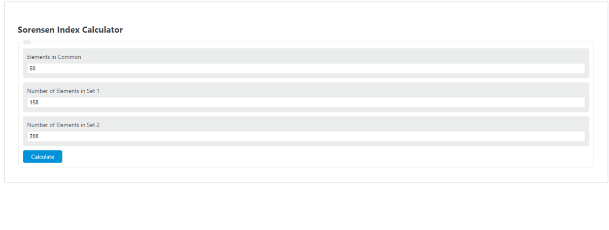
Calculate the Sorensen-Dice similarity index from species counts, lists, or abundances to compare overlap and shared species between two samples.
- ICC (Intraclass Correlation) Calculator
- All Biology Calculators
- Class Width Calculator
- Frequency Density Calculator
- Class Size Calculator
Sorensen Index Formula
The Sorensen Index is calculated using the following equation:
- SI is the Sorensen Index (ranges from 0 to 1)
- C is the number of elements (species, features, tokens) shared by both sets
- S1 is the total number of elements in Set 1
- S2 is the total number of elements in Set 2
The factor of 2 in the numerator means shared elements are counted twice, once for each set. This gives the Sorensen Index a higher baseline value than the Jaccard Index for the same data, making communities appear more similar. The two are mathematically linked: SI = 2J / (1 + J), where J is the Jaccard coefficient.
What is the Sorensen Index?
The Sorensen Index, formally called the Sorensen-Dice Coefficient, is a set-based similarity statistic that measures what fraction of all elements across two groups is shared between them. The result is a value between 0 (no overlap) and 1 (identical composition). It is a presence-absence metric, meaning it only asks whether an element exists in a set, not how abundant or frequent it is.
The index was independently derived twice. American zoologist Lee Raymond Dice introduced it in 1945 while studying ecological associations between mammal species. Danish botanist Thorvald Julius Sorensen (1902-1973) published a closely related formulation in 1948 in his landmark paper on grouping plant communities on Danish commons, applying it to presence-absence species lists from grassland surveys. Despite Dice preceding Sorensen by three years, the ecology literature most commonly refers to it as the Sorensen coefficient, while computer science and machine learning fields tend to use the Dice coefficient name.
Interpreting Sorensen Index Values
There are no universal cutoffs, but the following benchmarks reflect common usage across ecology and applied data science:
| Sorensen Index | Interpretation | Typical Context |
|---|---|---|
| 0.80 – 1.00 | Very high similarity | Same habitat surveyed twice; nearly identical species pools |
| 0.60 – 0.79 | High similarity | Adjacent habitats of the same type; closely related document sets |
| 0.40 – 0.59 | Moderate similarity | Related habitat types; some shared species or features |
| 0.20 – 0.39 | Low similarity | Different habitat types within the same region |
| 0.00 – 0.19 | Very low or no similarity | Cross-biome comparisons; entirely unrelated datasets |
In medical image segmentation, a Dice score above 0.70 is generally considered acceptable for automated algorithms, with values above 0.85 considered strong performance. In ecological beta diversity studies comparing sites within the same biome, values typically range from 0.40 to 0.75, with within-plot repeatability surveys often exceeding 0.80.
Sorensen Index Across Fields
Few similarity metrics have crossed disciplinary boundaries as widely as the Sorensen-Dice coefficient. Its simplicity and symmetry have made it a default tool across several distinct domains.
Ecology and Biodiversity
The Sorensen Index is a foundational tool in community ecology for measuring beta diversity, which is the variation in species composition across sites or time periods. A high Sorensen value between two plots indicates low beta diversity (similar communities), while a low value signals high turnover. Restoration ecologists use it to track whether a recovering site is converging toward a target reference community over time; progressive increases in the index signal successful restoration. Conservation planners apply it to evaluate potential habitat corridors, since a high Sorensen score between a protected area and an adjacent candidate buffer suggests the buffer supports compatible fauna. Researchers also calculate it before and after invasion events to quantify how much an invasive species has displaced native community composition.
Bioinformatics and Microbiome Research
In bioinformatics, the Sorensen coefficient compares gene sets, protein interaction networks, and microbial community profiles. When samples are represented as binary presence-absence vectors of operational taxonomic units (OTUs), the index captures compositional similarity between microbiomes. It is particularly favored in 16S rRNA amplicon studies because its higher baseline for shared taxa reflects the biological reality that many core gut microbiome members appear across most healthy individuals. Feature selection pipelines for biomarker discovery also use it to assess the reproducibility of selected gene sets across bootstrap replicates: a Sorensen score above 0.7 between two bootstrap runs suggests the feature selection is stable.
Natural Language Processing
In NLP and information retrieval, the Sorensen-Dice coefficient measures token-level overlap between text strings or documents. When applied to character bigrams, it handles spelling variation and transliterations well, performing competitively against edit-distance metrics on fuzzy deduplication tasks. Document retrieval systems use it to compare keyword sets between a query and indexed documents. Unlike TF-IDF cosine similarity, it makes no assumptions about term frequency, making it a fast, lightweight baseline for binary bag-of-words models where speed matters more than nuanced ranking.
Medical Image Segmentation
The Dice score has become the dominant evaluation metric in medical image segmentation, quantifying the spatial overlap between a predicted segmentation mask and a ground-truth annotation. Because a segmentation mask is a binary set of pixels or voxels, the overlap problem is structurally identical to comparing species presence lists. The Dice loss (1 minus the Dice score) is widely used as a differentiable training objective for U-Net and transformer-based segmentation architectures. Benchmarks such as BraTS for brain tumor segmentation report mean Dice scores as the primary metric, with top-performing models reaching above 0.89 for whole-tumor segmentation on MRI scans.
Beta Diversity: Turnover vs. Nestedness
A key ecological insight, formalized by ecologist Andres Baselga, is that Sorensen dissimilarity (1 minus the Sorensen Index) can be partitioned into two additive components: species turnover and nestedness.
The turnover component (beta_sim, also called Simpson dissimilarity) captures genuine species replacement: different species occurring at each site with similar total richness. The nestedness component (beta_nes) captures situations where the species pool at the poorer site is a strict subset of those at the richer site. Two pairs of sites can show identical Sorensen dissimilarity for completely different reasons: one pair may have high turnover (two distinct communities of equal richness), while another has high nestedness (one site is impoverished relative to the other). This distinction has direct conservation implications. High turnover between sites argues for protecting both independently, since they represent genuinely different biological assemblages. High nestedness may instead indicate that one site has suffered habitat degradation or resource loss, making restoration a more appropriate intervention than parallel protection.
Sorensen Index vs. Jaccard Index
The Sorensen and Jaccard indices answer the same similarity question but weight shared elements differently. Jaccard is defined as J = C / (S1 + S2 – C), where the denominator is the union of both sets. Sorensen is SI = 2C / (S1 + S2), where the denominator is the sum of both set sizes. The mathematical relationship is SI = 2J / (1 + J), which guarantees that the Sorensen index is always greater than or equal to the Jaccard index for the same data; they are equal only when both equal 0 or both equal 1.
As a concrete example: two sites each containing 20 species with 10 in common yield Jaccard = 10 / 30 = 0.333 and Sorensen = 20 / 40 = 0.500. The Sorensen index is higher because it weights shared species twice rather than counting them once against a larger union denominator. Neither index is objectively better; the choice depends on whether the research question emphasizes the shared fraction of an average set (Sorensen) or the shared fraction of the combined pool (Jaccard). Ecologists tend to prefer Sorensen for community comparison, while computational biologists and data scientists often default to Jaccard.
Limitations and When to Use Alternatives
The Sorensen Index has three core limitations. First, it is purely a presence-absence metric and ignores element abundance. Two communities where a shared species dominates carry the same score as one where it is rare. When count or biomass data are available and ecologically meaningful, the Bray-Curtis dissimilarity index is a better choice because it incorporates relative abundances. Second, the index gives equal weight to all elements regardless of importance: a keystone predator and a rare annual grass contribute equally to the score. Third, it provides no information about the internal structure of each community, such as evenness or dominance patterns. Pairing the Sorensen Index with Shannon-Wiener or Simpson diversity indices gives a more complete picture of community differences beyond simple compositional overlap.
In NLP contexts, the index is sensitive to tokenization granularity. Applied to whole words it behaves differently than when applied to character bigrams, and users should test both strategies before selecting one for a deduplication or retrieval pipeline. When sequence order or structural alignment matters, edit-distance metrics such as Levenshtein distance are typically more informative.