Convert electrical conductivity to resistivity or resistivity to conductivity using reciprocal formulas, with S/m, S/cm, µS/cm, Ω·m, Ω·cm, and micro-ohm units.
- All Unit Converters
- Materials Properties Unit Converters
- Resistivity Calculator
- Conductivity To Tds Calculator
Conductivity to Resistivity Formula
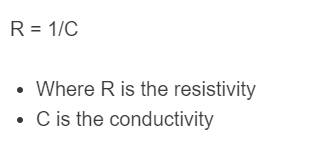
Electrical conductivity (σ) and resistivity (ρ) are inversely related properties of a material. Conductivity quantifies how easily electric current flows through a substance, while resistivity quantifies how strongly the substance opposes current flow. The conversion between them is:
And equivalently:
- ρ (rho) is the resistivity in ohm-meters (Ω·m)
- σ (sigma) is the conductivity in siemens per meter (S/m)
This reciprocal relationship means a material with a conductivity of 5.96 x 10⁷ S/m (copper at 20 °C) has a resistivity of 1.68 x 10⁻⁸ Ω·m. The relationship holds regardless of the unit system, though both values must be expressed in compatible units before dividing.
Conductivity and Resistivity Units
The SI unit of resistivity is the ohm-meter (Ω·m), but in practice several other units appear regularly depending on the field. In metallurgy, resistivity is often stated in nanoOhm-meters (nΩ·m) or microOhm-centimeters (μΩ·cm), since metals have extremely small resistivity values and these units avoid unwieldy scientific notation. For conductivity, the SI unit is siemens per meter (S/m), but megaSiemens per meter (MS/m) is standard in metals testing.
Water quality and environmental science typically use microSiemens per centimeter (μS/cm) or milliSiemens per centimeter (mS/cm) for conductivity, since solution conductivities are many orders of magnitude lower than those of metals. Soil scientists and geophysicists often report resistivity directly in Ω·m because subsurface resistivity spans a wide range from roughly 1 Ω·m for saturated clay to over 10,000 Ω·m for dry granite.
Common unit relationships: 1 S/cm = 100 S/m. 1 μΩ·cm = 1 x 10⁻⁸ Ω·m. 1 MS/m = 1 x 10⁶ S/m.
The IACS Scale
In 1913, the International Electrochemical Commission established the International Annealed Copper Standard (IACS) as a benchmark for electrical conductivity. Under this system, the conductivity of commercially pure annealed copper was assigned a value of 100% IACS, which corresponds to 58.0 MS/m (or equivalently a resistivity of 17.241 nΩ·m at 20 °C). Every other material is then expressed as a percentage of that copper benchmark.
Silver actually exceeds the copper standard at approximately 106% IACS, making it the most conductive element. Aluminum sits near 61% IACS, gold near 70% IACS, and brass alloys range from roughly 25% to 37% IACS depending on zinc content. The IACS scale remains widely used in quality control for wire, cable, and busbar manufacturing because it implicitly assumes a measurement temperature of 20 °C, eliminating a common source of ambiguity.
To convert from %IACS to S/m, multiply the IACS percentage by 580,000. To convert from S/m to %IACS, multiply the conductivity value by 1.7241 x 10⁻⁶.
Resistivity and Conductivity of Common Materials at 20 °C
The table below lists the resistivity, conductivity, and approximate %IACS values for a selection of metals, semiconductors, and insulators at 20 °C. These values are representative; actual measurements depend on purity, grain structure, alloying elements, and cold work.
| Material | Resistivity (Ω·m) | Conductivity (S/m) | %IACS |
|---|---|---|---|
| Metals | |||
| Silver | 1.59 x 10⁻⁸ | 6.30 x 10⁷ | ~106 |
| Copper (annealed) | 1.72 x 10⁻⁸ | 5.80 x 10⁷ | 100 |
| Gold | 2.44 x 10⁻⁸ | 4.10 x 10⁷ | ~70 |
| Aluminum | 2.65 x 10⁻⁸ | 3.77 x 10⁷ | ~61 |
| Calcium | 3.36 x 10⁻⁸ | 2.98 x 10⁷ | ~51 |
| Tungsten | 5.60 x 10⁻⁸ | 1.79 x 10⁷ | ~31 |
| Zinc | 5.90 x 10⁻⁸ | 1.69 x 10⁷ | ~29 |
| Nickel | 6.99 x 10⁻⁸ | 1.43 x 10⁷ | ~25 |
| Iron | 9.71 x 10⁻⁸ | 1.03 x 10⁷ | ~18 |
| Platinum | 1.06 x 10⁻⁷ | 9.43 x 10⁶ | ~16 |
| Tin | 1.09 x 10⁻⁷ | 9.17 x 10⁶ | ~16 |
| Lead | 2.20 x 10⁻⁷ | 4.55 x 10⁶ | ~8 |
| Titanium | 4.20 x 10⁻⁷ | 2.38 x 10⁶ | ~4 |
| Stainless Steel (304) | 6.90 x 10⁻⁷ | 1.45 x 10⁶ | ~2.5 |
| Nichrome | 1.10 x 10⁻⁶ | 9.09 x 10⁵ | ~1.5 |
| Semiconductors | |||
| Germanium | 4.6 x 10⁻¹ | 2.17 | n/a |
| Silicon | 6.4 x 10² | 1.56 x 10⁻³ | n/a |
| Insulators | |||
| Glass | 10¹⁰ to 10¹⁴ | 10⁻¹⁴ to 10⁻¹⁰ | n/a |
| Rubber (hard) | ~10¹³ | ~10⁻¹³ | n/a |
| Quartz (fused) | 7.5 x 10¹⁷ | 1.3 x 10⁻¹⁸ | n/a |
| Aqueous Solutions (approximate) | |||
| Ultrapure Water | 1.82 x 10⁵ | 5.5 x 10⁻⁶ | n/a |
| Drinking Water | 20 to 200 | 0.005 to 0.05 | n/a |
| Seawater | ~0.2 | ~5 | n/a |
| Values are approximate at 20 °C. Semiconductor values are for intrinsic (undoped) material. Actual values vary with purity, temperature, and doping. | |||
Material Classification by Resistivity Range
The resistivity of known materials spans more than 30 orders of magnitude, from about 10⁻⁸ Ω·m for the best metallic conductors to over 10²⁴ Ω·m for perfect insulators like PTFE. Engineers classify materials into three broad categories based on where they fall on this scale:
Conductors (resistivity below roughly 10⁻⁵ Ω·m): Metals and their alloys. Free electrons in the conduction band allow current to flow with minimal opposition. Silver, copper, and aluminum are the workhorses of electrical infrastructure.
Semiconductors (resistivity from about 10⁻⁵ to 10⁶ Ω·m): Materials like silicon and germanium whose conductivity can be tuned by many orders of magnitude through doping with impurities. Intrinsic silicon has a resistivity near 640 Ω·m, but heavily doped silicon used in integrated circuits can have a resistivity as low as 5 x 10⁻⁴ Ω·m.
Insulators (resistivity above roughly 10⁶ Ω·m): Materials that strongly resist current flow. Glass, ceramics, rubber, and most polymers fall in this range. These materials are essential as dielectrics in capacitors and as protective coatings on wires and circuit boards.
Temperature Dependence of Resistivity
Resistivity is not a fixed property; it changes with temperature. For most metals, resistivity increases approximately linearly with temperature over moderate ranges. This relationship is expressed as:
- ρ₀ is the resistivity at reference temperature T₀ (usually 20 °C)
- α is the temperature coefficient of resistivity (in K⁻¹ or °C⁻¹)
- T is the actual temperature
Metals have positive temperature coefficients, meaning their resistivity rises as temperature increases. This happens because thermal vibrations in the crystal lattice scatter conduction electrons more frequently, reducing the mean free path between collisions. Copper has a temperature coefficient of about 0.00393 per °C, so heating a copper conductor from 20 °C to 80 °C increases its resistivity by roughly 24%.
Semiconductors behave in the opposite direction. Their resistivity decreases with rising temperature because thermal energy promotes more electrons from the valence band into the conduction band. This negative temperature coefficient is the basis of thermistors used in temperature sensing circuits.
Some specialized alloys such as constantan (55% Cu, 45% Ni) and manganin (86% Cu, 12% Mn, 2% Ni) are engineered to have near-zero temperature coefficients. These alloys are used in precision resistors and measurement instruments where stable resistance over a range of operating temperatures is critical.
| Material | α (per °C at 20 °C) | Behavior |
|---|---|---|
| Silver | 0.0038 | Positive (metal) |
| Copper | 0.00393 | Positive (metal) |
| Aluminum | 0.00429 | Positive (metal) |
| Gold | 0.0034 | Positive (metal) |
| Iron | 0.00651 | Positive (metal) |
| Tungsten | 0.0045 | Positive (metal) |
| Platinum | 0.003927 | Positive (metal) |
| Nichrome | 0.0004 | Very low positive |
| Constantan | 0.000008 | Near zero |
| Manganin | 0.000002 | Near zero |
| Silicon | -0.075 | Negative (semiconductor) |
| Germanium | -0.048 | Negative (semiconductor) |
| Values are approximate. The linear model is accurate for metals over moderate temperature ranges (roughly -50 °C to 150 °C). | ||
Practical Applications
Electrical wiring and power transmission. Copper (resistivity 1.72 x 10⁻⁸ Ω·m) dominates building wiring, while aluminum (2.65 x 10⁻⁸ Ω·m) is preferred for overhead power lines because its lower density makes it cheaper per unit conductance per unit weight. Silver is used only in niche applications like high-frequency RF contacts where the slight conductivity advantage justifies the cost.
Water quality monitoring. Conductivity measurements in water are used as a proxy for total dissolved solids (TDS). Ultrapure water used in pharmaceutical manufacturing and semiconductor fabrication has a resistivity of approximately 18.2 MΩ·cm (0.055 μS/cm conductivity), while typical tap water ranges from 200 to 800 μS/cm. Seawater averages around 50,000 μS/cm. A sudden change in the conductivity of a water supply is a reliable early indicator of contamination or chemical discharge.
Geophysical surveying. Electrical resistivity tomography (ERT) maps subsurface geology by injecting current through electrodes and measuring the resulting voltage distribution. Saturated clay might read 1 to 10 Ω·m, wet sand 10 to 100 Ω·m, and dry granite over 10,000 Ω·m. Archaeologists use the same technique to detect buried foundations and voids without excavation.
Electronics and sensor design. Platinum resistance temperature detectors (RTDs) exploit platinum’s predictable and stable temperature coefficient (0.003927 per °C) to measure temperatures with precision of 0.01 °C or better. Thermistors made from semiconductor oxides use the large negative temperature coefficient of those materials for fast, sensitive temperature sensing in consumer electronics, automotive systems, and medical devices.
Metallurgy and quality control. Eddy current conductivity meters measure %IACS to verify alloy composition, detect heat treatment errors, and identify counterfeit materials. A batch of 6061-T6 aluminum should read about 40 to 43% IACS; a reading outside that range signals an incorrect alloy or an improper temper.
Conductivity to Resistivity Conversion Table
| Conductivity (S/m) | Resistivity (Ω·m) |
|---|---|
| 1 x 10⁻⁸ | 1 x 10⁸ |
| 1 x 10⁻⁶ | 1 x 10⁶ |
| 1 x 10⁻⁴ | 1 x 10⁴ |
| 0.001 | 1,000 |
| 0.01 | 100 |
| 0.05 | 20 |
| 0.1 | 10 |
| 0.5 | 2 |
| 1 | 1 |
| 5 | 0.2 |
| 10 | 0.1 |
| 100 | 0.01 |
| 1,000 | 0.001 |
| 10,000 | 1 x 10⁻⁴ |
| 1 x 10⁵ | 1 x 10⁻⁵ |
| 1 x 10⁶ | 1 x 10⁻⁶ |
| 1 x 10⁷ | 1 x 10⁻⁷ |
| 5.80 x 10⁷ (copper) | 1.72 x 10⁻⁸ |
| 6.30 x 10⁷ (silver) | 1.59 x 10⁻⁸ |
| ρ = 1/σ. All values exact by the reciprocal relationship. | |
FAQ
Conductivity measures how easily a material allows electric current to flow, while resistivity measures how strongly the material opposes current. They are exact reciprocals of each other: if you know one, you divide 1 by that value to get the other. Conductivity is measured in siemens per meter (S/m) and resistivity in ohm-meters (Ω·m).
In metals, increasing temperature causes atoms in the crystal lattice to vibrate more intensely, scattering conduction electrons more frequently and increasing resistivity. In semiconductors, the opposite happens: higher temperatures excite more electrons into the conduction band, increasing conductivity and decreasing resistivity. Specialized alloys like constantan and manganin are formulated to have nearly zero temperature dependence for use in precision instruments.
IACS stands for International Annealed Copper Standard. It is a conductivity scale where 100% IACS equals the conductivity of pure annealed copper, defined as 58.0 MS/m (5.80 x 10⁷ S/m) at 20 °C. To convert %IACS to S/m, multiply the percentage by 580,000. For example, aluminum at 61% IACS has a conductivity of 61 x 580,000 = 35,380,000 S/m, or about 3.54 x 10⁷ S/m.
Silver has the lowest resistivity of any element at room temperature, approximately 1.59 x 10⁻⁸ Ω·m at 20 °C, giving it a conductivity of about 6.30 x 10⁷ S/m (roughly 106% IACS). Despite this, copper is far more commonly used in electrical wiring because it costs significantly less per kilogram while offering nearly equivalent performance at 1.72 x 10⁻⁸ Ω·m.
Conductivity in water correlates directly with the concentration of dissolved ions. Ultrapure water has a resistivity of about 18.2 MΩ·cm, while tap water typically ranges from 200 to 800 μS/cm and seawater averages around 50,000 μS/cm. Water treatment plants, environmental agencies, and semiconductor fabrication facilities all use conductivity readings as a fast, continuous indicator of dissolved solids, contamination events, or process purity.