Calculate deadweight loss from Q1, Q2, P1, and P2, or solve for any missing value using the standard DWL triangle formula in markets.
Related Calculators
- Consumer Surplus Calculator
- Economics Multiplier Calculator
- Cost Efficiency Calculator
- Optimal Price Calculator (Best Sell Price)
- All Business Calculators
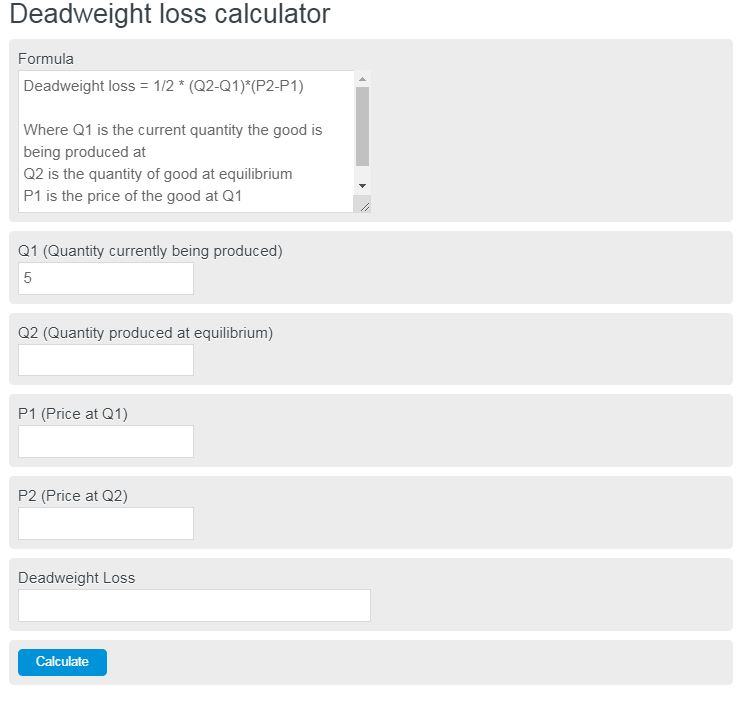
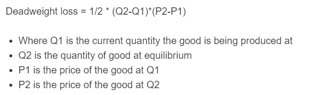
Deadweight Loss Formula
The calculator uses the standard deadweight loss triangle formula. It treats deadweight loss as one-half of the price wedge multiplied by the quantity gap.
Rearranged formulas are used when you leave one of the inputs blank:
- DWL = deadweight loss, measured in total currency value
- Q1 = quantity actually produced or traded under the distortion
- Q2 = efficient or competitive equilibrium quantity
- P1 = supply price or marginal cost at Q1
- P2 = demand price or willingness to pay at Q1
- |P2 – P1| = absolute price wedge
- |Q2 – Q1| = absolute quantity gap
If you enter Q1, Q2, P1, and P2, the calculator solves for deadweight loss. If you enter DWL and leave one variable blank, it rearranges the same triangle formula to solve for the missing value.
For Q1 and Q2, the calculator uses the common assumption that the efficient quantity is greater than or equal to the distorted quantity, so Q2 ≥ Q1. For P1 and P2, it uses the common assumption that willingness to pay is greater than or equal to marginal cost at Q1, so P2 ≥ P1.
Deadweight Loss Inputs and Interpretation
| Input | What it represents | Typical source |
|---|---|---|
| Q1 | Quantity traded after a tax, quota, monopoly restriction, price control, or other distortion | Observed market quantity or problem statement |
| Q2 | Quantity that would be traded at the efficient competitive equilibrium | Supply and demand intersection |
| P1 | Marginal cost or supply price at the distorted quantity | Supply curve value at Q1 |
| P2 | Willingness to pay or demand price at the distorted quantity | Demand curve value at Q1 |
Common Deadweight Loss Cases
| Situation | Why DWL occurs | How to identify Q1 and Q2 |
|---|---|---|
| Tax | The tax creates a wedge between the buyer price and seller price, reducing trade | Q1 is after-tax quantity, Q2 is no-tax equilibrium quantity |
| Quota | The quantity limit prevents some mutually beneficial trades | Q1 is quota quantity, Q2 is competitive equilibrium quantity |
| Monopoly | The firm restricts output below the competitive level | Q1 is monopoly quantity, Q2 is efficient quantity where price equals marginal cost |
| Price control | A binding price ceiling or floor reduces the amount traded | Q1 is the actual traded quantity, Q2 is the equilibrium quantity without the control |
Example
Example 1: Calculate deadweight loss
Suppose the distorted quantity is 80 units and the efficient quantity is 120 units. At Q1, the supply price is $10 and the demand price is $18.
The deadweight loss is $160.
Example 2: Solve for the efficient quantity
Suppose DWL is $90, Q1 is 50 units, P1 is $12, and P2 is $18.
The efficient quantity is 80 units.
FAQ
What does deadweight loss measure?
Deadweight loss measures the lost total surplus caused by an inefficient market outcome. It is the value of trades that would have benefited both buyers and sellers but do not happen because of a distortion such as a tax, quota, monopoly restriction, or binding price control.
Why does the formula use one-half?
The basic deadweight loss area is usually drawn as a triangle on a supply and demand graph. The area of a triangle is one-half times its base times its height. In this formula, the quantity gap is the base and the price wedge is the height.
Can deadweight loss be negative?
No. Deadweight loss is reported as a nonnegative value because it measures the size of lost surplus. The calculator uses absolute values for the price wedge and quantity gap, so the result is positive as long as there is a nonzero price wedge and a nonzero quantity gap.