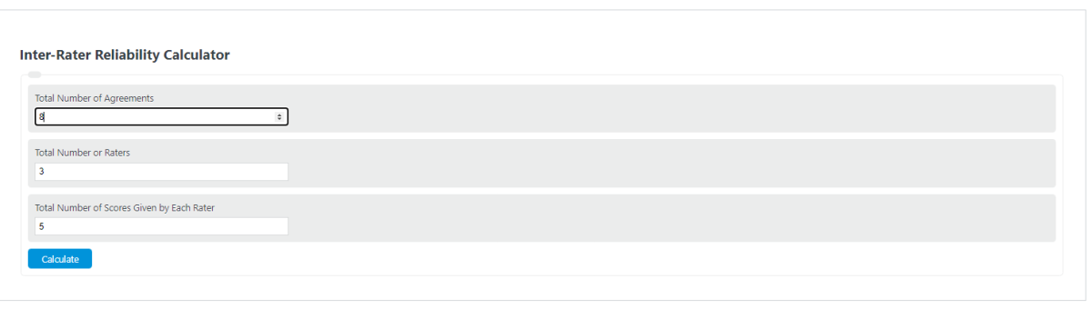
Enter the number of ratings in agreement, the total number of ratings, and the number of raters into the calculator to determine the inter-rater reliability.
- All Statistics Calculators
- Cronbach Alpha Calculator
- Sigma Level Calculator
- Average Rating Calculator (Star Rating)
- System Reliability Calculator
What Is Inter-Rater Reliability?
Inter-rater reliability (IRR) quantifies the degree to which independent raters, judges, or coders produce consistent assessments when evaluating the same set of subjects or items. It is one of the foundational quality checks in any study that relies on human judgment, from clinical diagnosis to content analysis to machine learning annotation pipelines. A high IRR value signals that the measurement instrument and rating criteria are well-defined enough that different observers reach the same conclusions independently.
IRR is distinct from intra-rater reliability, which measures the consistency of a single rater over time. Both fall under the broader umbrella of measurement reliability, but inter-rater reliability specifically addresses whether a construct can be rated consistently across people, not just within one person’s repeated attempts.
Percent Agreement Formula
The simplest measure of IRR is percent agreement, which the calculator above computes directly. The formula is:
Percent Agreement = (Number of agreements / Total number of ratings) x 100
This metric is intuitive and easy to compute, but it has a critical flaw: it does not account for agreement that would occur purely by chance. If two raters are classifying items into two categories, random guessing alone would produce roughly 50% agreement. Percent agreement cannot distinguish between genuine consensus and statistical coincidence, which is why chance-corrected measures like Cohen’s Kappa are preferred in published research.
Cohen’s Kappa
Jacob Cohen introduced this statistic in 1960 specifically to address the chance-agreement problem in percent agreement. Cohen’s Kappa is designed for exactly two raters classifying items into mutually exclusive nominal categories. The formula is:
k = (P_o – P_e) / (1 – P_e)
Where P_o is the observed proportion of agreement and P_e is the expected proportion of agreement under chance. P_e is calculated from the marginal totals of the raters’ classification matrix. Kappa values range from -1 to 1: a value of 1 indicates perfect agreement, 0 indicates agreement no better than chance, and negative values indicate systematic disagreement between the raters.
For ordinal or interval-scaled categories, Weighted Kappa extends the basic formula by assigning partial credit for near-misses. Linear weights penalize disagreements proportionally to their distance apart, while quadratic weights penalize proportionally to the square of the distance. Quadratic-weighted kappa is mathematically equivalent to the intraclass correlation coefficient under certain conditions, which makes it a useful bridge between categorical and continuous agreement measures.
Fleiss’ Kappa
Published by Joseph Fleiss in 1971, Fleiss’ Kappa generalizes the chance-corrected agreement framework to any fixed number of raters assigning nominal categories. Unlike Cohen’s Kappa, which compares two specific raters cell by cell, Fleiss’ Kappa works by computing the proportion of all rater pairs that agree for each item, then averaging across items and comparing to chance expectation. It does not require that the same individual raters evaluate every item, only that the same number of raters score each item. This makes it practical for studies where raters rotate across subjects, which is common in large-scale annotation projects.
Intraclass Correlation Coefficient (ICC)
When ratings are continuous or measured on an interval/ratio scale (e.g., pain scores from 0 to 10, or time measurements), kappa-based measures are inappropriate. The intraclass correlation coefficient (ICC) fills this role. ICC partitions the total variance in ratings into variance due to the subjects being rated and variance due to differences among raters. A high ICC means most of the variability comes from genuine differences between subjects rather than from rater inconsistency.
McGraw and Wong (1996) defined 10 forms of ICC based on three factors: the model (one-way random, two-way random, or two-way mixed effects), the type (single measures or average measures), and the definition (consistency or absolute agreement). The most commonly reported forms in research are ICC(2,1) for single-measure absolute agreement under a two-way random model, and ICC(3,1) for single-measure consistency under a two-way mixed model. Choosing the wrong form can substantially alter the reported reliability, so the specific ICC form should always be stated explicitly in any publication.
Krippendorff’s Alpha
Developed by Klaus Krippendorff, this coefficient is the most flexible IRR measure available. It handles any number of raters, works across nominal, ordinal, interval, and ratio data, tolerates missing data (raters do not need to score every item), and applies a small-sample correction. When there are no missing values and the data are nominal, Krippendorff’s Alpha produces values nearly identical to Fleiss’ Kappa. Its main advantage is generality: a single metric can be applied consistently regardless of the study design, eliminating the need to switch between different statistics for different data types.
Choosing the Right IRR Measure
The correct statistic depends on three factors: the number of raters, the measurement scale, and whether chance correction is needed.
For two raters with nominal categories, use Cohen’s Kappa. For two raters with ordinal categories, use Weighted Kappa (quadratic weights). For three or more raters with nominal categories, use Fleiss’ Kappa or Krippendorff’s Alpha. For continuous or interval/ratio data with any number of raters, use ICC. If there are missing data or mixed measurement levels, Krippendorff’s Alpha is the safest default. Simple percent agreement should only be used for quick exploratory checks, never as the sole reported statistic in formal research.
Interpreting Kappa Values
The most cited benchmark is the Landis and Koch (1977) scale: below 0.00 is poor agreement, 0.00 to 0.20 is slight, 0.21 to 0.40 is fair, 0.41 to 0.60 is moderate, 0.61 to 0.80 is substantial, and 0.81 to 1.00 is almost perfect. An alternative scale by Cicchetti (1994) classifies below 0.40 as poor, 0.40 to 0.59 as fair, 0.60 to 0.74 as good, and 0.75 to 1.00 as excellent.
Both scales are based on expert opinion rather than statistical derivation, and neither accounts for the number of categories, number of raters, or prevalence distribution. A kappa of 0.65 in a two-category scheme is not directly comparable to a kappa of 0.65 in a ten-category scheme. These benchmarks are useful as rough guidelines, but any serious reliability report should present the full confusion matrix, marginal distributions, and category-specific agreement rates alongside the summary kappa value.
The Kappa Paradox
Cohen’s Kappa has a well-documented counterintuitive behavior known as the kappa paradox, first described by Feinstein and Cicchetti in 1990. There are two forms. In the first, two raters can achieve very high percent agreement (e.g., 95%) yet produce a very low or even negative kappa. This happens when one category dominates the distribution (high prevalence), inflating the expected chance agreement so much that the observed agreement barely exceeds it. In the second form, two datasets with identical percent agreement can yield very different kappa values depending on how balanced the marginal distributions are.
The paradox is especially relevant in medical diagnostics and rare-event coding, where one category (e.g., “disease absent”) vastly outnumbers the other. In these situations, prevalence-adjusted and bias-adjusted kappa (PABAK) or Gwet’s AC1 may provide more stable estimates. Researchers should report prevalence indices and bias indices alongside kappa to help readers evaluate whether the paradox is distorting results.
Typical IRR Values by Field
Published kappa values vary widely across disciplines and tasks, which helps contextualize what a “good” score means in practice. In radiology, studies of chest X-ray interpretation commonly report kappa values between 0.40 and 0.75, reflecting the subjective nature of image reading. Dermatology diagnostic agreement for melanoma classification typically falls between 0.50 and 0.70. In psychiatry, structured clinical interviews using the DSM produce kappa values ranging from 0.50 to 0.80 depending on the diagnosis, with personality disorders at the lower end and major depressive episodes at the upper end.
In content analysis and natural language processing, annotation tasks for sentiment generally achieve kappa values of 0.70 to 0.85, while more subjective tasks like sarcasm detection often fall between 0.30 and 0.55. Machine learning data labeling pipelines routinely use IRR thresholds of 0.80 or higher before accepting annotated datasets for model training. In educational testing, essay scoring rubrics typically target ICC values of 0.70 to 0.90 for acceptable inter-rater consistency.
Improving Low Inter-Rater Reliability
Low IRR scores almost always trace back to ambiguous rating criteria, insufficient rater training, or a mismatch between the construct and the measurement scale. The most effective intervention is calibration training, where raters independently score a shared set of anchor items, discuss disagreements, and refine the coding rules until agreement reaches an acceptable threshold before the main study begins. Providing detailed scoring rubrics with concrete examples of borderline cases reduces subjective interpretation. Reducing the number of categories (when scientifically justified) also increases agreement, since finer-grained scales introduce more opportunities for disagreement. Finally, measuring IRR at multiple time points during data collection can catch rater drift, where a rater’s interpretation of the criteria gradually shifts over time.