Arc Elasticity Calculator - Calculator Academy

Reviewed By: Scott Hickam (MBA, Finance)

Enter the demand and price of a good or service at two different points to calculate the arc elasticity.

Arc Elasticity Formula

The arc elasticity formula (also called the midpoint elasticity formula) measures the responsiveness of quantity demanded to a price change between two observed points on a demand curve:

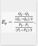
Where Ep is the arc elasticity coefficient, Q1 and Q2 are the quantities demanded at two observed points, and P1 and P2 are the corresponding prices. The denominator uses the average (midpoint) of both price and quantity rather than the initial value alone, which is the defining feature that separates this method from simple percentage change calculations.

What Is Arc Elasticity

Arc elasticity is a method for measuring the price elasticity of demand between two discrete points on a demand curve rather than at a single point. It was first proposed by Hugh Dalton in 1920 as an interpretation of Alfred Marshall's earlier elasticity framework, then refined by R.G.D. Allen in a 1934 paper published in The Review of Economic Studies. Allen's version, which uses the midpoint of both price and quantity as the base for percentage changes, became the standard because it satisfies three mathematical properties simultaneously: symmetry (the elasticity value is the same whether measured from point A to B or B to A), unit independence (the result does not change with the unit of measurement), and the revenue test (the coefficient equals exactly 1 when total revenue is identical at both points).

The practical significance of that symmetry property is substantial. Without it, measuring a price increase from $4 to $6 yields a different elasticity than measuring a price decrease from $6 to $4, even though the same two points are involved. The midpoint formula eliminates this inconsistency entirely, making arc elasticity the preferred tool when analyzing price changes that are not infinitesimally small.

Arc Elasticity vs. Point Elasticity

Point elasticity calculates demand responsiveness at a single exact point on a demand curve using the derivative of the demand function. It requires knowledge of the demand equation itself (for example, Qd = 200 - 5P) and computes elasticity as (dQ/dP) x (P/Q). Arc elasticity, by contrast, requires only two price-quantity observations and no underlying equation. This distinction matters in practice because real businesses rarely know their exact demand function but frequently observe sales data at two different price levels.

Point elasticity is more precise for very small price changes because it measures the instantaneous rate of change. Arc elasticity becomes less precise as the distance between the two measured points increases, since it averages over a larger section of the curve and cannot capture nonlinear behavior within that range. For price changes under roughly 5%, the two methods produce nearly identical results. For changes of 20% or more, they can diverge meaningfully, especially on convex demand curves.

Interpreting Arc Elasticity Values

The absolute value of the arc elasticity coefficient determines the demand classification and its implications for pricing strategy and revenue:

|Ed| > 1 (Elastic demand): Quantity demanded changes by a larger percentage than price. A 10% price increase causes more than a 10% drop in quantity. Total revenue moves in the opposite direction of price, so price cuts increase revenue and price hikes reduce it. Goods in this range include restaurant meals (typically 1.5 to 2.3), airline tickets purchased in advance (around 1.5 to 1.7), and brand-name consumer electronics.

|Ed| = 1 (Unit elastic demand): The percentage change in quantity exactly matches the percentage change in price. Total revenue remains constant regardless of the direction of the price change. This is the theoretical revenue-maximizing point for a monopolist.

|Ed| < 1 (Inelastic demand): Quantity demanded changes by a smaller percentage than price. A 10% price increase causes less than a 10% drop in quantity. Total revenue moves in the same direction as price, so price increases raise revenue. Common examples include gasoline in the short run (around 0.2 to 0.3), prescription medications (0.1 to 0.4), and tobacco products (roughly 0.3 to 0.5).

|Ed| = 0 (Perfectly inelastic): Quantity demanded does not change at all when price changes. This is theoretically rare but approximated by goods with no substitutes in the short term, such as insulin for Type 1 diabetics or emergency epinephrine.

|Ed| approaching infinity (Perfectly elastic): Any price increase above the market price causes quantity demanded to drop to zero. This occurs in perfectly competitive markets where buyers can instantly switch to identical substitutes at the prevailing price, such as commodity wheat sold at a grain exchange.

Empirical Elasticity Values by Industry

The following compiled values represent typical arc elasticity ranges observed in published economic studies. These values vary by region, time period, income level, and availability of substitutes, but they provide a useful reference for pricing analysis:

Highly inelastic (|Ed| below 0.5): Salt (0.1), water utility service (0.1 to 0.3), gasoline short-run (0.2 to 0.3), tobacco (0.3 to 0.5), electricity short-run (0.2 to 0.4), prescription drugs (0.1 to 0.4), funeral services (0.1 to 0.2).

Moderately inelastic (|Ed| 0.5 to 1.0): Coffee (0.5 to 0.8), housing short-run (0.6 to 0.8), public transportation (0.5 to 0.7), beer (0.7 to 0.9), gasoline long-run (0.6 to 0.8), medical services (0.5 to 0.8).

Elastic (|Ed| above 1.0): Restaurant meals (1.5 to 2.3), foreign travel (1.5 to 4.0), specific automobile brands (1.5 to 2.5), fresh fruit (1.0 to 1.5), furniture (1.0 to 1.5), luxury clothing (1.5 to 2.0), streaming entertainment subscriptions (1.0 to 1.8).

A key pattern in this data is that the time horizon matters enormously. Short-run gasoline elasticity (0.2 to 0.3) is roughly one-third of its long-run value (0.6 to 0.8) because consumers need time to adjust behavior by purchasing more fuel-efficient vehicles, moving closer to work, or switching to public transit.

Arc Elasticity and Total Revenue

The relationship between arc elasticity and total revenue (TR = P x Q) is one of the most directly actionable outputs of the calculation. When demand is elastic (|Ed| > 1), lowering the price increases total revenue because the percentage gain in quantity sold exceeds the percentage revenue lost per unit. When demand is inelastic (|Ed| < 1), raising the price increases total revenue because the smaller percentage loss in quantity is more than offset by the higher price per unit. At unit elasticity (|Ed| = 1), total revenue is at its maximum and does not change with small price movements in either direction.

This framework is the basis for revenue-based pricing decisions in industries ranging from airlines (which segment elastic leisure travelers from inelastic business travelers using advance-purchase requirements) to pharmaceuticals (where inelastic demand for essential medications allows price increases without proportional volume loss) to e-commerce platforms (which use A/B pricing tests to empirically estimate arc elasticity across product categories).

Extending the Midpoint Method Beyond Price

The midpoint (arc) formula can be applied to any two-variable elasticity relationship, not just price and quantity demanded. Cross-price arc elasticity replaces P with the price of a related good to measure how demand for one product responds to price changes in another. A positive cross-price arc elasticity indicates substitutes (beef and chicken, Uber and taxi), while a negative value indicates complements (printers and ink, cars and gasoline). Income arc elasticity replaces P with consumer income to classify goods as normal (positive coefficient) or inferior (negative coefficient), with luxury goods typically showing income elasticity above 1.0 and necessities falling between 0 and 1.0.

Supply-side arc elasticity applies the same formula to the quantity supplied rather than quantity demanded, measuring how producer output responds to price changes. Agricultural products tend to have very low short-run supply elasticity because planting cycles are fixed, while manufactured goods with scalable production lines show higher values.

Limitations

Arc elasticity assumes a roughly linear demand curve between the two measured points. If the actual curve is highly convex or concave over that interval, the midpoint average will overstate or understate the true elasticity at any given point within the range. This error grows with the distance between the two observations. Additionally, the method assumes all other factors (income, preferences, prices of substitutes and complements) remain constant between the two measurements. In practice, months or years may separate the two data points, during which multiple variables shift simultaneously, making it difficult to isolate the price-quantity relationship. Regression analysis on larger datasets is generally more reliable than two-point arc elasticity for formal demand estimation.

FAQ

What is arc elasticity?

Arc elasticity is a measure of the responsiveness of quantity demanded (or supplied) to a change in price, calculated between two distinct points on a demand or supply curve using the midpoint of both variables as the base for percentage changes. It was formalized by R.G.D. Allen in 1934 and is the standard method taught in introductory and intermediate economics courses for analyzing non-infinitesimal price changes.

When should I use arc elasticity instead of point elasticity?

Use arc elasticity when you have two observed price-quantity data points and do not know the underlying demand equation. It is the better choice for price changes larger than about 5%, where the direction of measurement (increase vs. decrease) would produce different results under simple percentage change methods. Use point elasticity when you have a known demand function and need precision at a specific price level.

Why is arc elasticity usually negative?

Arc elasticity for demand is typically negative because of the law of demand: as price increases, quantity demanded decreases (and vice versa). The numerator and denominator of the formula carry opposite signs, producing a negative quotient. Many textbooks and calculators report the absolute value for convenience, but the sign itself carries information. A positive arc elasticity of demand would indicate a Giffen good or Veblen good, both of which are rare exceptions to standard demand behavior.

How does arc elasticity relate to total revenue?

If |Ed| > 1 (elastic), a price decrease increases total revenue and a price increase decreases it. If |Ed| < 1 (inelastic), a price increase raises total revenue. At |Ed| = 1 (unit elastic), total revenue is maximized and does not change with small price shifts. This revenue test is built into the mathematical properties of the midpoint formula itself and is one of the three criteria Allen used to justify it over earlier arc elasticity measures.