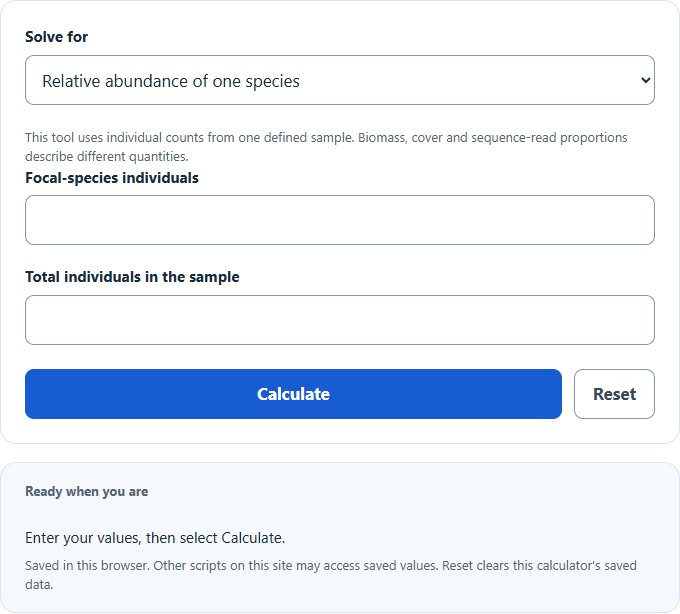
Calculate a species’ relative abundance or count, or analyze a community table with percentages, dominant species, richness, Shannon, Simpson, and evenness.
- All Biology Calculators
- Species Richness Calculator
- Basal Area Calculator
- NDVI Calculator
- Berger-Parker Index Calculator
Relative Abundance Formula
The following formula is used to calculate the relative abundance of a particular species within a community.
- Where RAi is the relative abundance of species i (%)
- ni is the number of individuals of species i
- N is the total number of individuals of all species in the community
To calculate relative abundance, divide the number of individuals of the species of interest by the total number of individuals in the community, then multiply by 100. The result can also be expressed as a decimal proportion (0 to 1) by omitting the multiplication step, which is the form used in most diversity index formulas.
What Is Relative Abundance?
Relative abundance is the proportional representation of a species within a biological community. It answers the question: of all organisms present in a defined habitat, what fraction belongs to species i? While species richness counts how many different species exist in an area, relative abundance captures how evenly individuals are distributed among those species. Two forests could each contain 10 tree species, but if one forest is 90% dominated by a single species while the other splits its population roughly equally, the ecological dynamics differ enormously.
Ecologists measure relative abundance using counts of individuals, biomass, percent cover, or frequency of occurrence depending on the organism and habitat. For mobile animals, mark-recapture or transect counts are standard. For sessile organisms like corals or plants, percent cover within quadrats is often more practical. The choice of measurement unit can shift relative abundance values: a single large oak tree may dominate by biomass but represent only a small fraction by individual count.
Relative Abundance and Biodiversity Indices
Relative abundance is the core input variable for nearly every quantitative biodiversity metric. The proportion pi = ni / N feeds directly into the following indices:
Shannon Diversity Index (H’): Calculated as H’ = -SUM(pi * ln(pi)) across all species. For S positive-count species, natural-log H′ ranges from 0 to ln(S), with higher values indicating greater diversity at comparable sampling and taxonomic resolution. A community where all species share equal relative abundance produces the maximum possible H’ for that species count.
Simpson’s Diversity Index (D): Calculated as D = SUM(pi2). This is the same-species probability for independent draws with replacement from the entered proportions. A finite-sample without-replacement estimator instead uses Σnᵢ(nᵢ−1)/[N(N−1)]; the calculator uses the proportion form. The complement (1 – D) or reciprocal (1/D) is often used so that higher values correspond to higher diversity. Simpson’s index is more sensitive to dominant species, while Shannon’s index is more sensitive to rare species.
Pielou’s Evenness (J’): Defined as J’ = H’ / ln(S), where S is species richness. This metric isolates the evenness component from diversity by normalizing Shannon’s index against its theoretical maximum. A J’ of 1.0 means perfectly even distribution; values approaching 0 indicate extreme dominance by one or a few species.
Berger-Parker Index (d): Simply the relative abundance of the single most dominant species: d = nmax / N. This simple dominance measure is affected by sampling variation and detectability. If several species tie for the largest count, the maximum proportion is shared; the calculator reports the tie. Values range from 1/S (perfect evenness) to 1.0 (complete monoculture).
Species Abundance Distribution Models
When relative abundances for all species in a community are plotted, many observed communities show a hollow-curve pattern, with numerous rare species and fewer common ones; this is not a universal law. Ecologists have developed several mathematical models to describe these species abundance distributions (SADs):
Geometric Series (Motomura Model): Assumes each successive species preempts a constant fraction of remaining resources. For a finite set of S ranks with total N, normalized expected abundance is ar = N * k * (1 – k)(r-1) / [1 – (1 – k)S], for 0 < k < 1. Without that denominator, the first S ranks sum to less than N. This preemption model is a hypothesis, not proof of a resource mechanism. This produces the steepest rank-abundance curve and fits species-poor, harsh environments like early-successional habitats, hot springs, or heavily polluted sites where 1 to 3 species dominate.
Log-Series (Fisher’s Alpha): Predicts that the number of species with n individuals is alpha * xn / n, where alpha is a diversity parameter and x is a fitted constant near 1. The log-series fits communities where many species are represented by just one individual (singletons). Fisher’s alpha remains relatively stable across sample sizes, making it a widely used diversity metric in tropical entomology and marine ecology.
Log-Normal Distribution: Proposed by Preston (1948), this model assumes that log-transformed abundances follow a normal (Gaussian) distribution. In practice, small samples reveal only the right tail of this distribution (the veil line effect), and more species appear as sampling increases. The log-normal fits many large, mature, species-rich communities and is the most commonly observed pattern in comprehensive surveys.
Broken Stick (MacArthur Model): Models resource partitioning as if a stick of length N is broken at S-1 random points, producing S segments. This often gives a relatively even reference distribution, but perfectly equal counts are the maximum-evenness case. Real communities rarely match broken stick predictions exactly, but it serves as a resource-partitioning reference model rather than a universal maximum-evenness model.
Rank-Abundance Curves
A rank-abundance curve (also called a Whittaker plot) graphs species from most to least abundant on the x-axis, with log-scaled relative abundance on the y-axis. This single visualization encodes both species richness (the length of the curve along the x-axis) and evenness (the slope of the curve). A steep, short curve indicates a low-diversity community dominated by few species. A long, gently sloping curve indicates high richness with relatively even abundance.
Different SAD models produce characteristic curve shapes. The geometric series appears as a straight descending line on a log-abundance plot. The log-normal produces a sigmoidal (S-shaped) curve. The broken stick model yields the shallowest slope. Comparing observed data with theoretical curves can generate hypotheses about community structure. Similar abundance patterns can arise from different mechanisms, so curve fit alone does not establish niche partitioning, neutral drift or environmental filtering.
Relative Abundance Across Ecosystems
Relative dominance varies among sites, taxa, sampling methods and units. A forest can be dominated by a few species by basal area while appearing more even by stem count. Coral cover, grassland plant counts and tree basal area cannot be compared as though they were the same count-based proportion. Use site-specific measurements rather than a universal ecosystem percentage benchmark.
A plankton sample may be dominated by a bloom species, while microbial sequence-read profiles describe a different measurement process. Read proportions are affected by extraction, gene-copy number and analytical methods and are not automatically proportions of individual organisms. This calculator accepts individual counts; using other weights requires changing the interpretation and validating the method separately.
Temporal Shifts in Relative Abundance
Relative abundance is not static. Seasonal cycles, disturbance events, climate change, and species invasions all cause species proportions to fluctuate. Tracking changes in relative abundance over time is a primary method for detecting population declines before a species disappears entirely. The Living Planet Index aggregates relative changes within monitored vertebrate populations over time. That population-trend index differs from one species’ share of all species in a community; it is not calculated by this widget.
When monitoring relative abundance across years, ecologists often normalize each species to a baseline year (nij / ni,baseline), producing a unitless index centered on 1.0. This differs from the cross-species relative abundance calculated above and is specifically designed to detect whether a given species is increasing or declining relative to its own historical population, rather than relative to other species in the community.
Sampling Bias and Detectability
Observed relative abundance values are always estimates subject to sampling effort and detection probability. Rare species are disproportionately underrepresented in small samples, a phenomenon known as the veil line in species abundance distributions. Additional quadrats, transects or trap-nights may reveal more rare species and may also change estimated proportions; the effect depends on the community and sampling design. Rarefaction curves and species accumulation curves help assess whether sampling has been sufficient to capture the community’s true abundance structure.
Detection probability also varies by species traits: cryptic, nocturnal, or highly mobile organisms are systematically undercounted relative to conspicuous, sedentary ones. Occupancy models and N-mixture models attempt to correct for imperfect detection by incorporating repeated surveys at the same site, separating the detection process from the underlying abundance process.
Practical Applications
Conservation biologists use relative abundance thresholds to prioritize species for protection. No universal 1% threshold establishes functional absence. Ecological function depends on species, interactions, absolute abundance and context; within-population decline and cross-species composition must be distinguished. Environmental impact assessments compare pre- and post-disturbance relative abundance profiles to quantify ecological damage. In fisheries management, shifts in relative abundance among commercial species signal changes in stock structure, ecosystem health, or the effectiveness of harvest regulations.
In microbiology and metagenomics, relative abundance calculated from DNA sequence reads is the standard output of 16S rRNA amplicon surveys and shotgun sequencing pipelines. Tools like QIIME2 and mothur generate relative abundance tables that form the basis for community composition analysis, differential abundance testing, and beta-diversity ordination across human gut, soil, aquatic, and clinical microbiome studies.
About Relative Abundance
Is relative abundance a percentage? Relative abundance is fundamentally a proportion (ranging from 0 to 1). It is frequently multiplied by 100 and reported as a percentage for intuitive interpretation, but the decimal form is the version used in diversity index calculations like Shannon’s H’ and Simpson’s D.
What is the difference between absolute and relative abundance? Absolute abundance is the total count (or estimated count) of individuals of a species in a defined area, such as 500 deer in a forest. Relative abundance is that count divided by the total count of all species, expressing how one species compares proportionally to the entire community. A species can increase in absolute abundance while declining in relative abundance if other species grow faster.
Can relative abundances for all species in a community exceed 100%? No. Because relative abundance is a proportion of the total, the sum of relative abundances across all species in a community must equal exactly 100% (or 1.0 in decimal form). Independently rounded percentages may differ slightly from 100%. The equality assumes mutually exclusive categories that exhaust the same denominator; overlapping cover or inconsistent totals require a different interpretation.
Why do most species have low relative abundance? This pattern, documented across virtually all taxa and ecosystems studied, arises from a combination of factors: limited niche space, competitive exclusion, stochastic population dynamics, and dispersal limitation. Neutral theory (Hubbell, 2001) proposes that much of this pattern can be explained by random demographic drift alone, without invoking species-specific ecological differences, though niche-based explanations remain important for many communities.